Custom dynamics

Import Python libraries

Hide code cell content

import logging

import qrules
import sympy as sp
from IPython.display import Markdown, Math
from matplotlib_inline.backend_inline import set_matplotlib_formats
from qrules.io import asmermaid

from ampform.io import aslatex

set_matplotlib_formats("svg")
logging.getLogger("qrules.transition").setLevel(logging.ERROR)  # hide progress bar

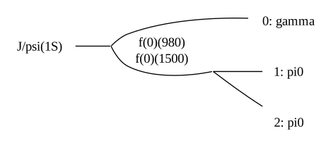
We start by generating allowed transitions for a simple decay channel, just like in Formulate amplitude model:

reaction = qrules.generate_transitions(
    initial_state=("J/psi(1S)", [+1]),
    final_state=[("gamma", [+1]), "pi0", "pi0"],
    allowed_intermediate_particles=["f(0)(980)", "f(0)(1500)"],
    allowed_interaction_types=["strong", "EM"],
    formalism="helicity",
)

Visualize allowed transitions

Hide code cell source

src = asmermaid(reaction, collapse_graphs=True, markdown=True)
Markdown(src)

        flowchart LR
    T0_0["$$0: \gamma$$"]
    T0_1["$$1: \pi^{0}$$"]
    T0_2["$$2: \pi^{0}$$"]
    T0_N0["$$J/\psi(1S)$$"]
    T0_N1@{ shape: text, label: " " }
    T0_3("$$\begin{gathered} f_{0}(980) \\\ f_{0}(1500) \end{gathered}$$")
    T0_N0 --- T0_3
    T0_3 --- T0_N1
    T0_N0 --- T0_0
    T0_N1 --- T0_1
    T0_N1 --- T0_2
    

Next, create a HelicityAmplitudeBuilder using get_builder():

from ampform import get_builder

model_builder = get_builder(reaction)

In Formulate amplitude model, we used DynamicsSelector.assign() with some standard lineshape builders from the builder module. These builders have a signature that follows the ResonanceDynamicsBuilder Protocol. Here it is, together with the implementation behind create_relativistic_breit_wigner(), which is the RelativisticBreitWignerBuilder.__call__() method of a RelativisticBreitWignerBuilder instance:

Show source code

Hide code cell source

import inspect
import textwrap

from IPython.display import Markdown

from ampform.dynamics.builder import (
    ResonanceDynamicsBuilder,
    create_relativistic_breit_wigner,
)

Markdown(f"""
```python
{inspect.getsource(ResonanceDynamicsBuilder)}

{textwrap.dedent(inspect.getsource(create_relativistic_breit_wigner))}
```
""")

class ResonanceDynamicsBuilder(Protocol):
    """Protocol that is used by `.DynamicsSelector.assign`.

    Follow this `~typing.Protocol` when defining a builder function that is to be used
    by `.DynamicsSelector.assign`. For an example, see the source code
    `.create_relativistic_breit_wigner`, which creates a `.SimpleBreitWigner`.

    .. seealso:: :doc:`/dynamics/custom`
    """

    def __call__(
        self, resonance: Particle, variable_pool: TwoBodyKinematicVariableSet
    ) -> BuilderReturnType:
        """Formulate a dynamics `~sympy.core.expr.Expr` for this resonance."""


def __call__(
    self, resonance: Particle, variable_pool: TwoBodyKinematicVariableSet
) -> BuilderReturnType:
    """Formulate a relativistic Breit–Wigner for this resonance."""
    if self.energy_dependent_width:
        expr, parameter_defaults = self.__energy_dependent_breit_wigner(
            resonance, variable_pool
        )
    else:
        expr, parameter_defaults = self.__simple_breit_wigner(
            resonance, variable_pool
        )
    if self.form_factor:
        form_factor, parameters = self.__create_form_factor(
            resonance, variable_pool
        )
        parameter_defaults.update(parameters)
        return form_factor * expr, parameter_defaults
    return expr, parameter_defaults

A function that behaves like a ResonanceDynamicsBuilder should return a tuple of some Expr (which formulates your lineshape) and a dict of Symbols to some suggested initial values. This signature is required so the builder knows how to extract the correct symbol names and their suggested initial values from a Transition.

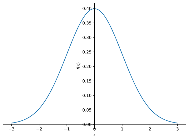
The Expr you use for the lineshape can be anything. Here, we use a Gaussian function and wrap it in a function. As you can see, this function stands on its own, independent of ampform:

def my_dynamics(x: sp.Symbol, mu: sp.Symbol, sigma: sp.Symbol) -> sp.Expr:
    return sp.exp(-((x - mu) ** 2) / sigma**2 / 2) / (sigma * sp.sqrt(2 * sp.pi))

x, mu, sigma = sp.symbols("x mu sigma")
sp.plot(my_dynamics(x, 0, 1), (x, -3, 3), axis_center=(0, 0))
my_dynamics(x, mu, sigma)

\[\displaystyle \frac{\sqrt{2} e^{- \frac{\left(- \mu + x\right)^{2}}{2 \sigma^{2}}}}{2 \sqrt{\pi} \sigma}\]

We can now follow the example of the create_relativistic_breit_wigner() to create a builder for this custom lineshape:

from qrules.particle import Particle

from ampform.dynamics.builder import TwoBodyKinematicVariableSet


def create_my_dynamics(
    resonance: Particle, variable_pool: TwoBodyKinematicVariableSet
) -> tuple[sp.Expr, dict[sp.Symbol, float]]:
    res_mass = sp.Symbol(f"m_{resonance.name}")
    res_width = sp.Symbol(f"sigma_{resonance.name}")
    expression = my_dynamics(
        x=variable_pool.incoming_state_mass,
        mu=res_mass,
        sigma=res_width,
    )
    parameter_defaults = {
        res_mass: resonance.mass,
        res_width: resonance.width,
    }
    return expression, parameter_defaults

Now, just like in Set dynamics, it’s simply a matter of plugging this builder into DynamicsSelector.assign() and we can formulate() a model with this custom lineshape:

for name in reaction.get_intermediate_particles().names:
    model_builder.dynamics.assign(name, create_my_dynamics)
model = model_builder.formulate()

As can be seen, the HelicityModel.parameter_defaults section has been updated with the some additional parameters for the custom parameter and there corresponding suggested initial values:

Math(aslatex(model.parameter_defaults))

\[\begin{split}\displaystyle \begin{aligned} m_{f(0)(980)} \;&=\; 0.99 \\ \sigma_{f(0)(980)} \;&=\; 0.06 \\ C_{J/\psi(1S) \to {f_{0}(980)}_{0} \gamma_{+1}; f_{0}(980) \to \pi^{0}_{0} \pi^{0}_{0}} \;&=\; 1+0i \\ m_{f(0)(1500)} \;&=\; 1.522 \\ \sigma_{f(0)(1500)} \;&=\; 0.108 \\ C_{J/\psi(1S) \to {f_{0}(1500)}_{0} \gamma_{+1}; f_{0}(1500) \to \pi^{0}_{0} \pi^{0}_{0}} \;&=\; 1+0i \\ \end{aligned}\end{split}\]

Let’s quickly have a look what this lineshape looks like. First, check which Symbols remain once we replace the parameters with their suggested initial values. These are the kinematic variables of the model:

expr = model.expression.doit().subs(model.parameter_defaults)
free_symbols = tuple(sorted(expr.free_symbols, key=lambda s: s.name))
free_symbols

(m_12, theta_0)

To create an invariant mass distribution, we should integrate out the \(\theta\) angle. This can be done with integrate():

m, theta = free_symbols
integrated_expr = sp.integrate(
    expr,
    (theta, 0, sp.pi),
    meijerg=True,
    conds="piecewise",
    risch=None,
    heurisch=None,
    manual=None,
)
Math(aslatex(integrated_expr.n(1), terms_per_line=1))

\[\begin{split}\displaystyle \begin{aligned} & 5.0 \cdot 10^{1} e^{- 277.777777777778 \left(m_{12} - 0.99\right)^{2}} \\ & \;+\; 2.0 \cdot 10^{1} e^{- 85.7338820301783 \left(m_{12} - 1.522\right)^{2}} \\ & \;+\; 6.0 \cdot 10^{1} e^{- 42.8669410150892 \left(m_{12} - 1.522\right)^{2}} e^{- 138.888888888889 \left(m_{12} - 0.99\right)^{2}} \\ \end{aligned}\end{split}\]

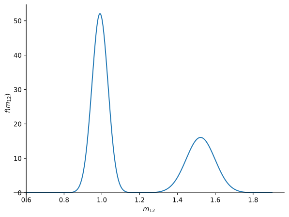
Finally, here is the resulting expression as a function of the invariant mass, with custom dynamics!

x1, x2 = 0.6, 1.9
sp.plot(integrated_expr, (m, x1, x2), axis_center=(x1, 0));