Inspect model interactively
In this notebook, we illustrate how to interactively inspect a HelicityModel. The procedure should in fact work for any sympy.Expr.
Create amplitude model
First, we create some HelicityModel. We could also have used pickle to load() the HelicityModel that we created in Formulate amplitude model, but the cell below allows running this notebook independently.
import qrules as q

from ampform import get_builder
from ampform.dynamics.builder import (
    create_non_dynamic_with_ff,
    create_relativistic_breit_wigner_with_ff,
)

result = q.generate_transitions(
    initial_state=("J/psi(1S)", [-1, +1]),
    final_state=["gamma", "pi0", "pi0"],
    allowed_intermediate_particles=["f(0)(980)", "f(0)(1500)"],
    allowed_interaction_types=["strong", "EM"],
    formalism_type="canonical-helicity",
)
model_builder = get_builder(result)
initial_state_particle = result.get_initial_state()[0]
model_builder.set_dynamics(initial_state_particle, create_non_dynamic_with_ff)
for name in result.get_intermediate_particles().names:
    model_builder.set_dynamics(name, create_relativistic_breit_wigner_with_ff)
model = model_builder.generate()
In this case, as we saw, the overall model contains just one intensity term \(I = |\sum_i A_i|^2\), with \(\sum_i A_i\) some coherent sum of amplitudes. We can extract \(\sum_i A_i\) as follows:
import sympy as sp

amplitude = model.expression.args[0].args[0].args[0]
assert isinstance(amplitude, sp.Add)
Substitute some of the boring parameters with the provided parameter_defaults:
substitutions = {
    symbol: value
    for symbol, value in model.parameter_defaults.items()
    if not symbol.name.startswith("Gamma_")
    and not symbol.name.startswith("m_")
}
amplitude = amplitude.doit().subs(substitutions)
Lambdify
We now need to identify the Symbol over which the amplitude is to be plotted. The remaining symbols will be turned into slider parameters.
plot_symbol = sp.Symbol("m_12", real=True)
slider_symbols = sorted(amplitude.free_symbols, key=lambda s: s.name)
slider_symbols.remove(plot_symbol)
slider_symbols
[Gamma_f(0)(1500),
 Gamma_f(0)(980),
 m_1,
 m_2,
 m_f(0)(1500),
 m_f(0)(980),
 phi_1+2,
 theta_1+2]
Next, lambdify() the expression:
np_amplitude = sp.lambdify(
    (plot_symbol, *slider_symbols),
    amplitude,
    "numpy",
)
We also have to define some functions that formulate what we want to plot. A pure amplitude won’t do, because we can only plot real values:
import numpy as np


def intensity(plot_variable, **kwargs):
    values = np_amplitude(plot_variable, **kwargs)
    return np.abs(values) ** 2


def argand(**kwargs):
    values = np_amplitude(plot_domain, **kwargs)
    argand = np.array([values.real, values.imag])
    return argand.T
Prepare sliders
Tip
This procedure has been extracted to the façade function symplot.prepare_sliders().
We also need to define the domain over which to plot, as well sliders for each of the remaining symbols. The function create_slider() helps creating a ipywidgets slider for each Symbol:
from symplot import create_slider

plot_domain = np.linspace(0.2, 2.5, num=400)
sliders_mapping = {
    symbol.name: create_slider(symbol) for symbol in slider_symbols
}
If the name of a Symbol is not a valid name for a Python variable (see str.isidentifier()), lambdify() ‘dummifies’ it, so it can be used as argument for the lambdified function. Since mpl_interactions.interactive_plot() works with these (dummified) arguments as identifiers for the sliders, we need some mapping between the Symbol and their dummified name. This can be constructed with the help of inspect.signature():
import inspect

symbols_names = list(map(lambda s: s.name, (plot_symbol, *slider_symbols)))
arg_names = list(inspect.signature(np_amplitude).parameters)
arg_to_symbol = dict(zip(arg_names, symbols_names))
The class SliderKwargs comes in as a handy manager for this dict of sliders:
from symplot import SliderKwargs

sliders = SliderKwargs(sliders_mapping, arg_to_symbol)
sliders
SliderKwargs(
  sliders={'Gamma_f(0)(1500)': FloatSlider(value=0.0, description='$\\Gamma_{f(0)(1500)}$'),
   'Gamma_f(0)(980)': FloatSlider(value=0.0, description='$\\Gamma_{f(0)(980)}$'),
   'm_1': FloatSlider(value=0.0, description='$m_{1}$'),
   'm_2': FloatSlider(value=0.0, description='$m_{2}$'),
   'm_f(0)(1500)': FloatSlider(value=0.0, description='$m_{f(0)(1500)}$'),
   'm_f(0)(980)': FloatSlider(value=0.0, description='$m_{f(0)(980)}$'),
   'phi_1+2': FloatSlider(value=0.0, description='$\\phi_{1+2}$'),
   'theta_1+2': FloatSlider(value=0.0, description='$\\theta_{1+2}$')},
  arg_to_symbol={'Dummy_1052': 'Gamma_f(0)(1500)',
   'Dummy_1051': 'Gamma_f(0)(980)',
   'm_1': 'm_1',
   'm_2': 'm_2',
   'Dummy_1050': 'm_f(0)(1500)',
   'Dummy_1049': 'm_f(0)(980)',
   'Dummy_1048': 'phi_1+2',
   'Dummy_1047': 'theta_1+2'},
)
SliderKwargs also provides convenient methods for setting ranges and initial values for the sliders.
n_steps = 100
sliders.set_ranges(
    {
        "m_f(0)(980)": (0.3, 1.8, n_steps),
        "m_f(0)(1500)": (0.3, 1.8, n_steps),
        "Gamma_f(0)(980)": (0.01, 1, n_steps),
        "Gamma_f(0)(1500)": (0.01, 1, n_steps),
        "m_1": (0.01, 1, n_steps),
        "m_2": (0.01, 1, n_steps),
        "phi_1+2": (0, 2 * np.pi, 40),
        "theta_1+2": (-np.pi, np.pi, 40),
    }
)
The method set_values() is designed in particular for parameter_defaults, but also works well with both argument names (that may have been dummified) and the original symbol names:
import qrules as q

pdg = q.load_pdg()
sliders.set_values(model.parameter_defaults)
sliders.set_values(
    {  # symbol names
        "phi_1+2": 0,
        "theta_1+2": np.pi / 2,
    },
    # argument names
    m_1=pdg["pi0"].mass,
    m_2=pdg["pi0"].mass,
)
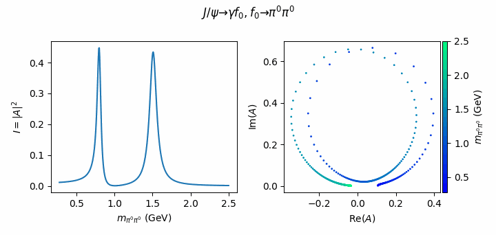
Interactive Argand plot
Finally, we can use mpl-interactions to plot the functions defined above with regard to the parameter values:
%matplotlib widget
import matplotlib.pyplot as plt
import mpl_interactions.ipyplot as iplt

# Create figure
fig, axes = plt.subplots(
    1, 2, figsize=0.9 * np.array((8, 3.8)), tight_layout=True
)
fig.suptitle(R"$J/\psi \to \gamma f_0, f_0 \to \pi^0\pi^0$")
ax_intensity, ax_argand = axes
m_label = R"$m_{\pi^0\pi^0}$ (GeV)"
ax_intensity.set_xlabel(m_label)
ax_intensity.set_ylabel("$I = |A|^2$")
ax_argand.set_xlabel("Re($A$)")
ax_argand.set_ylabel("Im($A$)")

# Fill plots
controls = iplt.plot(
    plot_domain,
    intensity,
    **sliders,
    slider_formats={slider: "{:.3f}" for slider in arg_names},
    ylim="auto",
    ax=ax_intensity,
)
iplt.scatter(
    argand,
    controls=controls,
    xlim="auto",
    ylim="auto",
    parametric=True,
    c=plot_domain,
    s=1,
    ax=ax_argand,
)
plt.colorbar(label=m_label, ax=ax_argand, aspect=30, pad=0.01)
plt.winter()
Tip
See Compare Breit-Wigner and K-matrix for why \(K\)-matrix dynamics are better than simple Breit-Wigners when resonances are close to each other.