K-matrix¶

While ampform does not yet provide a generic way to produce an amplitude model with \(K\)-matrix dynamics, it is fairly simple to produce an expression for the \(K\)-matrix and play around with it interactively.

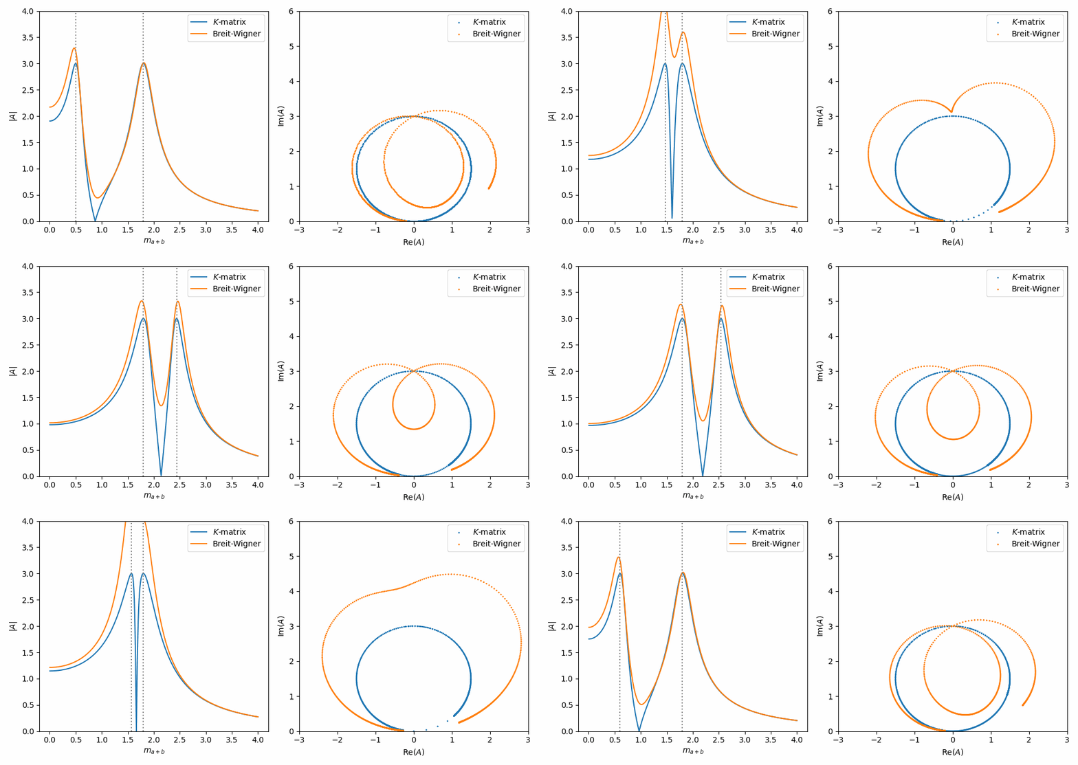
This notebook shows how a \(K\)-matrix for one channel with two poles compares to using a sum of two Breit-Wigner functions. For more info on the \(K\)-matrix, see this instructive presentation [Meyer 2018], or the classic paper [Chung et al. 1995].

Mass-dependent width¶

In both the \(K\)-matrix and the relativistic Breit-Wigner, it is important to use a mass-dependent width (also called running width). This width makes use of BlattWeisskopf barrier factors. Those factors depend on angular momentum \(L\), meson radius \(d\), and the masses of the decay products \(m_a\) and \(m_b\):

import sympy as sp

L = sp.Symbol("L", integer=True)
m_a, m_b = sp.symbols("m_a m_b")
d = 1  # meson radius / impact parameter

from ampform.dynamics.lineshape import BlattWeisskopf, breakup_momentum


def running_width(m, m0, gamma0):
    q = breakup_momentum(m, m_a, m_b)
    q0 = breakup_momentum(m0, m_a, m_b)
    form_factor = BlattWeisskopf(q, d, L)
    form_factor0 = BlattWeisskopf(q0, d, L)
    return (
        gamma0 * (m0 / m) * (form_factor ** 2 / form_factor0 ** 2) * (q / q0)
    )

m, m0, gamma0 = sp.symbols("m, m0, Gamma0")
q = breakup_momentum(m, m_a, m_b)
q0 = breakup_momentum(m0, m_a, m_b)
form_factor = BlattWeisskopf(q, d, L)
form_factor0 = BlattWeisskopf(q0, d, L)
running_width(m, m0, gamma0).subs(
    {
        form_factor ** 2: sp.Symbol("B^{2}_{L}(q)"),
        form_factor0 ** 2: sp.Symbol("B^{2}_{L}(q_0)"),
    },
).subs(
    {
        2 * q: sp.Symbol("q"),
        2 * q0: sp.Symbol("q0"),
    },
)

\[\displaystyle \frac{B^{2}_{L}(q) \Gamma_{0} m_{0} q}{B^{2}_{L}(q_0) m q_{0}}\]

Amplitude definition¶

A \(K\)-matrix for two poles and one channel reduces to the following:

def kmatrix_term(m, m1, gamma1, m2, gamma2):
    running_gamma1 = running_width(m, m1, gamma1)
    running_gamma2 = running_width(m, m2, gamma2)
    return (m1 * running_gamma1) / (
        (m1 ** 2 - m ** 2)
        - sp.I * m1 * running_gamma1
        - sp.I * (m1 ** 2 - m ** 2) / (m2 ** 2 - m ** 2) * m2 * running_gamma2
    )


a, b = sp.symbols("C_a C_b")
m, m1, m2, gamma1, gamma2 = sp.symbols("m, m1, m2, Gamma1, Gamma2")
term1 = kmatrix_term(m, m1, gamma1, m2, gamma2)
term2 = kmatrix_term(m, m2, gamma2, m1, gamma1)
kmatrix = a * term1 + b * term2

running_gamma1 = running_width(m, m1, gamma1)
running_gamma2 = running_width(m, m2, gamma2)
kmatrix.subs(
    {
        running_gamma1: sp.Symbol(R"\Gamma_{1}(m)"),
        running_gamma2: sp.Symbol(R"\Gamma_{2}(m)"),
    },
)

\[\displaystyle \frac{C_{a} \Gamma_{1}(m) m_{1}}{- i \Gamma_{1}(m) m_{1} - \frac{i \Gamma_{2}(m) m_{2} \left(- m^{2} + m_{1}^{2}\right)}{- m^{2} + m_{2}^{2}} - m^{2} + m_{1}^{2}} + \frac{C_{b} \Gamma_{2}(m) m_{2}}{- \frac{i \Gamma_{1}(m) m_{1} \left(- m^{2} + m_{2}^{2}\right)}{- m^{2} + m_{1}^{2}} - i \Gamma_{2}(m) m_{2} - m^{2} + m_{2}^{2}}\]

Two Breit-Wigner ‘poles’ with the same parameters would look like this (making use of relativistic_breit_wigner_with_ff():

from ampform.dynamics.lineshape import relativistic_breit_wigner_with_ff

term1 = relativistic_breit_wigner_with_ff(m, m1, gamma1, m_a, m_b, L, d)
term2 = relativistic_breit_wigner_with_ff(m, m2, gamma2, m_a, m_b, L, d)
bw = a * term1 + b * term2

running_gamma1 = running_width(m, m1, gamma1)
running_gamma2 = running_width(m, m2, gamma2)
ff = BlattWeisskopf(breakup_momentum(m, m_a, m_b), d, L)
bw.subs(
    {
        running_gamma1: sp.Symbol(R"\Gamma_{1}(m)"),
        running_gamma2: sp.Symbol(R"\Gamma_{2}(m)"),
        ff: sp.Symbol("B_{L}(q)"),
    },
)

\[\displaystyle \frac{B_{L}(q) C_{a} \Gamma_{1} m_{1}}{- i \Gamma_{1}(m) m_{1} - m^{2} + m_{1}^{2}} + \frac{B_{L}(q) C_{b} \Gamma_{2} m_{2}}{- i \Gamma_{2}(m) m_{2} - m^{2} + m_{2}^{2}}\]

Prepare sliders¶

Just like in Inspect model interactively, we use symplot to generate sliders for the Symbols in both expressions:

from symplot import prepare_sliders

np_kmatrix, sliders = prepare_sliders(kmatrix.doit(), m)
set(sliders)

{'C_a', 'C_b', 'Gamma1', 'Gamma2', 'L', 'm1', 'm2', 'm_a', 'm_b'}

Luckily, the dummy variables for the lambdified argument should be the same (the symbol names are valid identifiers), so as long as we use the same order of the positional arguments, we can lambdify() the sum of Breit-Wigners in the same way:

np_bw = sp.lambdify(
    (m, a, b, gamma1, gamma2, L, m1, m2, m_a, m_b),
    bw.doit(),
    "numpy",
)

Again, we need to identify how we want to plot these (complex) amplitudes:

def abs_amplitude_bw(plot_variable, **kwargs):
    values = np_bw(plot_variable, **kwargs)
    return np.abs(values)


def argand_bw(**kwargs):
    values = np_bw(plot_domain, **kwargs)
    argand = np.array([values.real, values.imag])
    return argand.T


def abs_amplitude_kmatrix(plot_variable, **kwargs):
    values = np_kmatrix(plot_variable, **kwargs)
    return np.abs(values)


def argand_kmatrix(**kwargs):
    values = np_kmatrix(plot_domain, **kwargs)
    argand = np.array([values.real, values.imag])
    return argand.T

We also need to define a domain over which to plot the invariant mass:

import numpy as np

plot_domain = np.linspace(0, 4, 1_000)

…as well as ranges and (optionally) initial values for the sliders:

sliders.set_ranges(
    C_a=(0, 5),
    C_b=(0, 5),
    m1=(0, 3, 100),
    m2=(0, 3, 100),
    Gamma1=(0, 2, 100),
    Gamma2=(0, 2, 100),
    m_a=(0, 1),
    m_b=(0, 1),
    L=(0, 8),
)
sliders.set_values(
    C_a=3,
    C_b=3,
    m1=1.2,
    m2=1.8,
    Gamma1=0.3,
    Gamma2=0.4,
    L=0,
)

Compare Breit-Wigner and K-matrix¶

That’s it. Now, we do the same as in Inspect model interactively, but with some slight adaptations to combine the \(K\)-matrix and Breit-Wigner formulations of both amplitudes in one plot. Notice in the Argand plot how the \(K\)-matrix preserves unitarity, while the Breit-Wigners do not!

%matplotlib widget
import matplotlib.pyplot as plt
import mpl_interactions.ipyplot as iplt

# Create figure
fig, axes = plt.subplots(
    1, 2, figsize=1.2 * np.array((8, 3.8)), tight_layout=True
)
# fig.suptitle(R"$J/\psi \to \gamma f_0, f_0 \to \pi^0\pi^0$")
ax_intensity, ax_argand = axes
m_label = "$m_{a+b}$"
ax_intensity.set_xlabel(m_label)
ax_intensity.set_ylabel("$|A|$")
ax_argand.set_xlabel("Re($A$)")
ax_argand.set_ylabel("Im($A$)")

# Intensity
controls = iplt.plot(
    plot_domain,
    abs_amplitude_kmatrix,
    label="$K$-matrix",
    **sliders,
    ylim="auto",
    ax=ax_intensity,
)
iplt.plot(
    plot_domain,
    abs_amplitude_bw,
    label="Breit-Wigner",
    controls=controls,
    ylim="auto",
    ax=ax_intensity,
)
plt.legend(loc="upper right")
iplt.axvline(controls["m1"], c="gray", linestyle="dotted")
iplt.axvline(controls["m2"], c="gray", linestyle="dotted")

# Argand plots
iplt.scatter(
    argand_kmatrix,
    label="$K$-matrix",
    controls=controls,
    parametric=True,
    s=1,
    ax=ax_argand,
)
iplt.scatter(
    argand_bw,
    label="Breit-Wigner",
    controls=controls,
    parametric=True,
    s=1,
    ax=ax_argand,
)
plt.legend(loc="upper right");

AmpForm

K-matrix¶

Mass-dependent width¶

Amplitude definition¶

Prepare sliders¶

Compare Breit-Wigner and K-matrix¶